Printer-friendly version

Easy Java Simulations: An Interactive Science Learning Tool
Fu-Kwun Hwang, National Taiwan Normal University
Francisco Esquembre, University of Murcia

Abstract
Easy Java Simulations (Ejs) is an interactive tool developed for the conceptual learning of science. Ejs is not designed for professional programmers, but for teachers and students who want to create (or modify) scientific simulations. With Ejs, they can concentrate their effort on writing and refining the relations in the underlying scientific model, and dedicate the minimum possible amount of time to the programming techniques. Teachers without programming experience have already created simulations for use in their curriculum after an introductory Ejs workshop. An alternative approach, and a very promising one, is to let students modify the model in a simulation or create their own simulations, thus engaging in what educational researchers call constructive modeling.

About the authors...

1. Introduction 
Successful technology-driven transformations have been seen in industry, business and research as a result of developments in computer hardware and software. Computer simulations have been used in all three sectors for many years. Initially, programs were designed to help do jobs more easily or quickly. Processes that take a very long time or happen very quickly are good candidates for simulations. Difficult, dangerous or expensive processes are also good candidates (Harper and Wright, 2002). Will information technology have a similarly successful impact on education? The answer depends on how the teaching and learning process integrates information technology. Students do not interact with the computer, but with a program. Research has shown that these programs must provide an activity or goal that leads to cognitive involvement. Computer simulations can help students to understand invisible conceptual worlds of science through animation, which can lead to more abstract understanding of scientific concepts. Quantitative data can be manipulated and visualized to help students form a qualitative mental picture. Such complex experiences can help students to identify patterns within simulations, and formulate explanations for phenomena in terms of models and theories. Simulations must not only allow learners to construct and manipulate screen “objects” for exploring underlying concepts, but they must also provide learners with the observation and manipulation tools necessary for exploring and testing hypotheses in the simulated world (Jonassen, 1996). Combined with graphical representations, simulations should allow the learner to visualize abstract concepts and to link them to prior knowledge, thereby fostering conceptual learning.

Computer simulations in an instructional context involve using the computer to model real-world phenomena in order to help students gain insights into the behavior of complex systems. Students interacting with an instructional simulation gain a better understanding of a real system, process or phenomenon by exploring concepts, testing hypotheses, and discovering explanations (Lunetta and Hofstein, 1991; Mellar and Bliss, 1993; Raghavan & Glaser, 1995). This interactivity provides opportunities for students to modify their mental models by comparing the outputs of the model with their expectations (Jackson et al., 1996), and to engage or motivate students to explore and couple actions with effects which will lead to understanding. Simulations can provide insight into the inner workings of a process – not just what happens, but also how and why. We all agree that the computer simulations are not a substitute for observation of and experimentation with real phenomena. Nevertheless, computer modeling with online simulations can add a valuable new dimension to scientific inquiry and understanding. Well-designed computer applications allow learners to use visual and kinesthetic resources to explore phenomena and to test theories so that they may eventually construct a web of connections between new information and information they already know.

Various simulations can be found on the internet. For example, hundreds of Java simulations were created at the National Taiwan Normal University (NTNU) Virtual Physics Laboratory. There are more than 76 mirror sites around the world. Many physics teachers use these Java simulations in their teaching. These simulations are adaptable to the extent that the user can change any pre-defined parameters. However, the interactive capabilities of these simulations are limited because the models are fixed. Teachers often ask for modifications in these simulations in order to adapt them to different student abilities or different pedagogic needs. Users with programming backgrounds have also asked for source code, so they can modify these simulations for their projects. Programming, however, is not an easy task for most teachers and students. For those who have limited programming experience, the simulations with an embedded model are readily manipulated. The users can learn from the outcome of the simulation, even if they might not know how the physics models were implemented in the simulation.

Creating a simulation by oneself requires an extra effort. The starting point is a full understanding of the phenomenon being simulated. But beyond an understanding of the physical model the instructor needs the programming and technical expertise to describe the phenomenon in computer language. With Ejs, the task of creating a simulation is greatly simplified. That is, the majority of the programming work is done by automatic code generation based upon text-based instructions and menu/mouse selections from the instructor creating the simulation. Java source code is generated automatically and compiled into class files. In addition, a jar file and the associated html page can be produced to view the simulation within a browser. This automatic code generation allows the Ejs user to concentrate on describing the model by defining the parameters related to the model, providing an equation for the evolution of these parameters, setting the constraints between variables, and building a graphical representation.

An additional advantage of using Ejs is that it causes the instructor who is building the simulation to think through the problem in a new way. Ejs is a media for making, doing and creating. Construction, simulation, visualization, and analytic description of the science model are linked during the creation process. We have found that, by creating a simulation, many teachers get a new perspective of the phenomenon they are trying to explain, which almost always increases their enthusiasm about the use of this technology with their students.

An external link to the Virtual Physics Laboratory.

An external link to the mirror sites.

2. Description of the Tool 
Easy Java Simulations is a software tool designed for the creation of computer simulations. A computer simulation is a computer program that reproduces a natural phenomenon through the visualization of the evolution of its state. Each state is described by a set of variables that change in time due to the iteration of a given algorithm. Ejs was developed for an Open Source Physics Project at the University of Murcia, Spain. Ejs, and the simulations created with it, can be used as independent programs under different operating systems, or be distributed via the internet and run within html pages by most popular web browsers.

What makes Ejs different from most other products is that Ejs is not designed to make life easier for professional programmers, but instead it was conceived by science teachers, for science teachers and students -- that is, for people who are more interested in the content of the simulation, the simulated phenomenon itself, and much less in the technical aspects needed to build the simulation program. Hence, Ejs provides a conceptual structure and simplified tools that allow designers to concentrate most of their time on the description of the model of the phenomenon they want to be simulated. The typical audience includes science students, teachers and researchers who have a basic knowledge of programming, but who cannot afford the big investment of time needed to create a complete graphical simulation. They may be able to describe the phenomena in their respective disciplines in terms of algorithms, but still need an extra effort to create a sophisticated, interactive graphical user interface.

Most computer simulations of scientific phenomena can be described in terms of the model-control-view paradigm. This paradigm states that a simulation is composed of three parts:

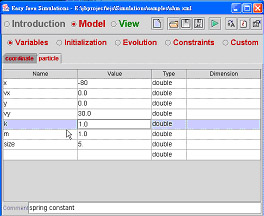
1. The model, which describes the phenomenon under study in terms of

• variables, that hold the different possible states of the phenomenon, and
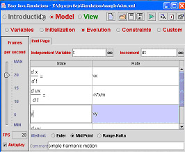
• relationships among these variables (corresponding to the laws that govern the phenomenon), expressed by computer algorithms.

2. The control, which defines certain actions that a user can perform on the simulation.

3. The view, which shows a graphical representation of the different states that the phenomenon can have. This representation can be done in a realistic or schematic form.
These three parts are deeply interconnected. The model obviously affects the view, since a change in the state of the model must be made graphically evident to the user. The control affects the model because control actions can (and usually do) modify the value of variables of the model. Finally, the view affects the model and the control, because the graphical interface can contain components that allow the user to modify variables or perform the predefined actions.

To further simplify the construction of a simulation, Ejs suppresses the control part, merging it half into the view, half into the model. Actually, modern computer programs are interactive, which means that the user can modify the program’s logic by doing some gestures (such as clicking or dragging the mouse, or hitting the keyboard) with the computer peripherals on the program’s interface (or view). Thus, the view itself can be used to control the simulation. On the other hand, if we want this interaction to have certain relevance within the program, these gestures on the interface need to trigger actions that affect the model’s variables. Therefore, the best place to define these actions is in the model itself.

Creating a simulation in Ejs consists in defining its model and its view (i.e., the GUI or graphical user interface) and establishing the mutual connections needed for

• the correct visualization of the state of the phenomenon being simulated and
• the appropriate interaction of the user with the view (either to modify this state or to perform the actions defined on the model).

This explicit separation in parts reinforces conceptually the central role of the model of a simulation. It is the model that defines what the program simulates and how. There may be different views for a given model. Teachers can create the same simulation with different GUIs for different tasks or different students.

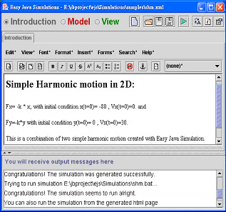
In addition to the Model and View, Ejs has one more component from which a simulation is built– the Introduction. For pedagogical or scientific purposes, it is always helpful to include a description of what a simulation does, including the instructions on how to operate it and other pertinent information. This information appears in the Introduction, which is used to generate the content of the html web page. Therefore, there are three major parts to the interface: Introduction, Model and View.

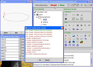
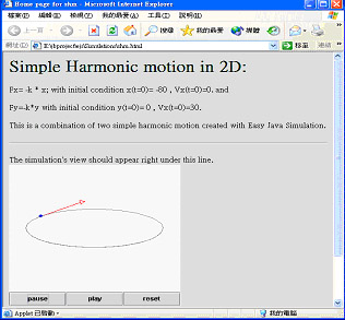
Figure 1 shows an example of the Introduction for a Simple Harmonic Motion (SHM) simulation. Figure 2 shows the SHM simulation that is created with Ejs.

Figure 1. Content in the Introduction will be used to generate Web pages for the simulation.

Screen capture movie (~2.4 MB) demonstrates creating the Web page content for the Simple Harmonic Motion (SHM) simulation using Introduction.

Figure 2. Java simulation embedded in web page created with Ejs.

Screen capture movie (~3.2 MB) shows a Java simulation embedded in a Web page.

The Model interface follows the Introduction, and has five sections:

1. Variables: As shown in Figure 3, all the variables for the simulation need to be predefined with specific data types (or dimensions for arrays). The initial value for the variables can be specified here or in the “initialization” section. Users can group the variables into several pages under different names. For example, the SHM simulation has two tabbed pages for the variables. The variables defined in the “coordinate” page are those that specify the boundary for the simulated region on the screen and the timing information in the simulation. The variables defined on the “particle” page are those that correspond to the position and velocity in the X-Y rectangular coordinate system, the mass for the simulated particle, and the spring constant for the SHM.

2. Initialization (optional): Different sets of initial conditions can be defined to simulate different cases for the same model (scientific phenomenon). Initial values for the array variables are usually initialized here.

3. Evolution: Figure 4 shows that the simulation will be created with 20 frames per second and that the “Mid Point” method is adopted for the numerical integration. The “Independent Variable” is t. When the user enters in the “State” column and in the “Rate” column,

is shown instead, in order to specify the evolution condition

Notice that the equation for simple harmonic motion is transformed into evolution conditions:

  becomes   
where m and k are mass and spring constants.

Simulations for different models can easily be created by modifying the equations with different forms.

4. Constraints (optional): Optional constraints or relations between variables can be defined here.

5. Custom (optional): Custom functions can be defined to be used in other sections in the Model or as a trigger action for the GUI in the View.

Figure 3. The variables for the SHM simulation.

Screen capture movie (~3.6 MB) demonstrates defining variables for the SHM simulation.

Figure 4. The evolution/constraints for variables.

Screen capture movie (~4 MB) demonstrates specifying the relationships of the variables for the SHM simulation using the Evolution page.

Physics teachers and students have found it is easy to follow the above steps to specify the mathematics in the model for the SHM simulation. These are the same steps they would use to describe SHM in their physics classes. A comparison between the two is shown in Table 1. It is this similarity that makes many science teachers feel, for the first time, they are able to create their own simulations with Ejs.

Steps to describe model for the simulation in Ejs

Steps to describe phenomenon in science class

Table 1. Comparisons between steps to describe a model for the simulation in Ejs and steps to describe the same phenomenon in science class.

Figure 5. Creating the GUI for the simulation in Ejs.

Screen capture movie (~5.8 MB) demonstrates creating the GUI for the SHM simulation in View.

As shown in Figure 5, Ejs provides an easy-to-use interface to create the GUI for the simulation. Interactive graphic elements can be built with mouse drag and drop actions. The tree-like structure of elements in the View is used to select and edit a particular element. Each element provides some characteristics for itself, called “Properties,” which can be linked with variables defined in the model. The linking mechanism is a two-way, dynamic process. At any moment, the property of the element will reflect whatever value the linked variable holds, and vice versa. If the property changes as a result of an interaction such as typing in a new value or moving a scrollbar, the variable will receive a new value. For example, the “X, Y, Size X and Size Y” properties for the arrow were set to link with variables x, y, vx and vy in the model. Whenever x, y, vx or vy are changed with time in the model during the simulation, an arrow in the user interface reflects the change. Also, some elements have properties of a special type, which are called “Actions,” to specify what to do when the user interacts with the element (e.g. Reset, Pause, Play). Once the Model and View have been completed, Ejs can generate the Java source code, compile the source to create class files, compress all the class files into a jar file and make html pages with a single mouse click. The generated simulations will automatically pop up on screen for inspection. If any error occurs in compiling the source code, extended information is provided to guide the user to check for the specific pages in the Model.

Screen capture movie (~3.9 MB) demonstrates generating the Java source code, compiling the source to create class files, compressing all the class files into a jar file and making html pages with a single mouse click.

We have had three 3-days workshops this year, showing high school science teachers (and some university faculty members) how to create their interactive teaching modules with Ejs. The first day focused on guidelines for developing instructional material using modern information technology, showing examples of well-established resources available in the internet, and giving a brief introduction to the Ejs. At the end of the first day, all the attendees were asked to bring in at least one simulation proposal they would like to create by themselves, and we promised to help them finish the task. The second day, attendees followed a step-by-step method with selected examples to create simulations with Ejs in the morning sessions. Then, they were asked to create their own simulations in the afternoon with our assistance. On the third day, all were asked to present their simulations for discussion and further improvement at the last session of the workshop. Teachers (many of them without programming experience) were successful in creating scientific simulations to be used in their curriculum.

Response from those teachers at workshops was very positive and resulted in our adding new features to Ejs from the teachers’ feedback. We have created a web version of the Ejs interface, so Ejs can be accessed via a browser (http://www.phy.ntnu.edu.tw/osejs/). With the web version interface, simulations created online were all saved at our server (with JavaScript/PHP/MySQL). Additionally, simulations created offline can be uploaded to our server and shared with others. Novices can study how others design their Model/View in Ejs to create a simulation. They can easily modify an existing simulation to create another simulation with a different model or view for their own purpose. A discussion forum is also available for users to exchange ideas or get help.

An external link to web version of the Ejs interface.

3. Future Work
Because there is an educational value in the process of creating a simulation, Ejs can also be used as a pedagogical tool itself. With it, teachers can ask their students to create a simulation by themselves, perhaps by following some guidelines provided by the teacher. This way, Ejs can help students make their concept of a phenomenon explicit. Used in groups, it can also improve students’ capabilities to discuss and communicate about science. An alternative approach, and a very promising one, is to let students create their own simulations, thus engaging in so called constructive modeling. This has the advantage of getting the student to do science in an exploratory and constructive way, achieving many of the recommended best-practices in the classroom. The next phase of this work will include having undergraduate students and some selected high school students create their own simulations using Ejs.

4. Acknowledgement
This work is supported by National Science Council. (NSC91-2511-S-003-057).

5. References
1. Barry Harper and Rob Wright (2002), Designing Simulations for complex skill development, Educational Multimedia and Hypermedia & Telecommunications, 2002, 713-718 , AACE.

2. Jackson, S. L., Stratford, S. J., Krajcik, J., and Soloway, E., 1996, A learner-centered tool for students building models, Communications of the ACM, 39(4), 48-49.

3. Jonassen, D. H. (1996). Computers in the classroom: Mindtools for critical thinking. Englewood Cliffs, NJ: Prentice-Hall, Inc.

4. Lunetta, V., & Hofstein, A. (1991). Simulation and laboratory practical activity. In B. Woodnough (Ed.), Practical science, 125-150. Miltonkeynes, PA: Open University Press.

5. Mellar, H. G., & Bliss, J. (1993). Expressing the student's concepts versus exploring the teacher's: Issues in the design of mociroworlds for teaching. Journal of Educational Computing Research, 9(1), 89-112.

6. Raghavan, K., & Glaser, R. (1995). Model-based analysis and reasoning in science: The MARS curriculum. Science Education, 79(1), 37-61.

7. NTNU Virtual Physics Laboratory (2002) http://www.phy.ntnu.edu.tw/java/ (77 mirror sites)

8. Easy Java Simulations (2002): http://fem.um.es/Ejs/ and http://www.phy.ntnu.edu.tw/osejs/

9. Open Source Physics Project : http://www.opensourcephysics.org/

********** End of Document **********

IMEJ multimedia team member assigned to this paper	Yue-Ling Wong

© 2003 Wake Forest University (from Volume 5, Number 2, of The Interactive Multimedia Electronic Journal of Computer-Enhanced Learning).